Model Quantization — What Actually Happens When You Shrink a Transformer

I first ran into quantization the hard way, trying to cram a DistilBERT checkpoint onto an iPhone for on-device inference. The tutorials made it sound simple: call a function, get a smaller model, ship it. What nobody mentioned was that "INT8" often quietly means "mostly INT8, with FP16 islands the toolchain left behind for safety." That experience pushed me to actually understand what quantization does under the hood, rather than trusting black-box APIs to make the right calls for me.
This is what I've learned since. Not from tutorials. From reading papers, breaking models, and staring at NVIDIA's documentation longer than I probably should have.
Why quantization matters
The arithmetic is brutal. If you store Llama 2 7B in FP16, each parameter occupies 2 bytes. That's roughly 14 GB just for the weights, before you account for activations, the KV cache, or the operating system's overhead. Most consumer GPUs tap out well before that.
Quantization reduces the precision of model parameters. Instead of 32-bit or 16-bit floating-point numbers, you represent weights (and sometimes activations) in 8-bit or even 4-bit formats. The model shrinks. Inference speeds up. Power consumption drops. But accuracy degrades, sometimes imperceptibly, sometimes catastrophically. Everything that follows is about navigating that trade-off.
Quantization isn't a magic compression switch — it's a set of deliberate trade-offs between bits, accuracy, and what your hardware can actually execute.
Floating-point formats
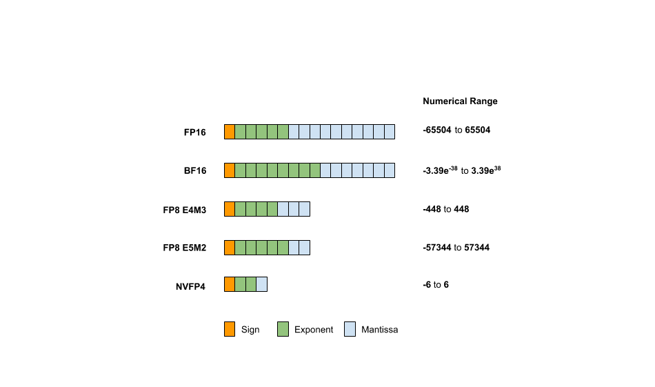
Before getting into how quantization works, it helps to understand what it's converting between. A floating-point number in any format is built from three components:
- Sign bit: one bit, 0 for positive, 1 for negative
- Exponent bits: define the range of representable values (the power of 2)
- Mantissa bits (significand): define the precision, how many distinct values exist within that range
The general formula for a floating-point value is:
Different formats allocate these bits differently, and that allocation completely determines what the format is good at:
| Format | Total Bits | Exponent | Mantissa | Approx Range |
|---|---|---|---|---|
| FP32 | 32 | 8 | 23 | |
| FP16 | 16 | 5 | 10 | |
| BF16 | 16 | 8 | 7 | |
| FP8 (E4M3) | 8 | 4 | 3 | |
| FP8 (E5M2) | 8 | 5 | 2 | |
| FP4 (E2M1) | 4 | 2 | 1 |
BF16 is worth pausing on. It keeps the same 8 exponent bits as FP32 (preserving range) but drops the mantissa to just 7 bits. That's why it became the default training format for large language models: the range matches FP32, and the reduced precision barely matters during gradient updates. FP8 E4M3 is the workhorse for inference quantization. Four exponent bits give you enough range, and 3 mantissa bits provide just enough precision that most model weights survive the conversion.
Three things you can quantize
Most people think of quantization as compressing model weights. That's the obvious target: weights are static, known ahead of time, and easy to map to lower precision. But there are two more components worth considering:
1. Weights
The static parameters of the model. Quantizing weights from FP16 to FP8 cuts memory roughly in half. For Llama 2 7B, that means going from ~14 GB to ~7 GB. The difference between needing an A100 and fitting on a consumer RTX 4090.
2. Activations
The intermediate outputs computed during inference, the values flowing between layers. These are dynamic (they change with every input), which makes them harder to quantize. But quantizing activations is where you get actual compute speedups, because modern tensor cores execute lower-precision math faster. Weight-only quantization saves memory. Activation quantization saves time.
3. KV Cache
Specific to transformer decoder models. During autoregressive generation, the KV cache stores key-value pairs from previous tokens to avoid redundant computation. For long sequences, this cache dominates memory usage. Llama 2 7B with a 4096-token context window can accumulate several gigabytes of KV cache. Quantizing it to FP8 or INT8 reclaims that memory without meaningfully hurting generation quality.
The quantization algorithm
Here's where the math gets concrete. Quantization maps a floating-point value to a low-precision value . There are two approaches, and the distinction matters more than most tutorials let on.
Affine (asymmetric) quantization
Affine quantization uses two parameters: a scale factor and a zero-point . The scale controls the step size between quantized levels. The zero-point ensures that real-valued 0.0 maps exactly to a quantized integer. This matters because neural network operators rely heavily on zero-padding.
The quantization formula:
Where:
- is the original floating-point value
- is the scale factor (positive real number)
- is the zero-point (integer, same type as )
- define the quantized range (e.g., to for INT8)
- maps to the nearest quantized level
- keeps values within the representable range
To recover the approximate original value (dequantization):
The hat on is doing a lot of work. It's reminding you that this is an approximation. The round-trip from to back to introduces rounding error and clipping error, both baked into the final model's accuracy.
Symmetric quantization
Symmetric quantization drops the zero-point entirely by fixing . This simplifies the math and eliminates the addition operations during inference:
The trade-off: symmetric quantization can waste representable range if your data distribution is skewed. One side of the number line gets allocated codes that never get used. But for most transformer weights, the distribution is roughly centred around zero, so symmetric quantization works well enough.
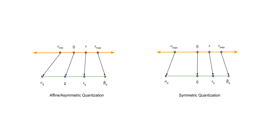
This is worth understanding intuitively. In affine quantization, real-valued zero can land anywhere on the quantized number line. In symmetric quantization, zero always maps to quantized zero. That simplicity is why NVIDIA's TensorRT and Model Optimizer both default to symmetric: the accuracy difference is marginal, and the computational savings are real.
The AbsMax algorithm
The scale factor is central to the entire process. Get it wrong and you either waste precision (scale too large) or clip important values (scale too small). The most common method for computing it is AbsMax quantization, which is almost embarrassingly simple:
Where is the maximum absolute value in the data being quantized, and is the maximum representable quantized value.
For a concrete example, mapping FP16 values to FP8 E4M3 (where ):
Once you have , quantizing any value is just:
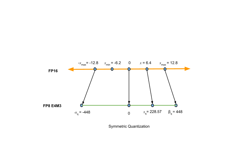
AbsMax is popular because it's fast and requires no calibration data. But it has an obvious vulnerability: outliers. A single extreme value in a weight tensor inflates the scale factor, wasting precision for all the other values. This is the motivation for the advanced algorithms I'll cover shortly.
Quantization granularity
Even with a good algorithm, you need to decide how to share quantization parameters across a tensor. This choice, the granularity, often matters more than the algorithm itself.
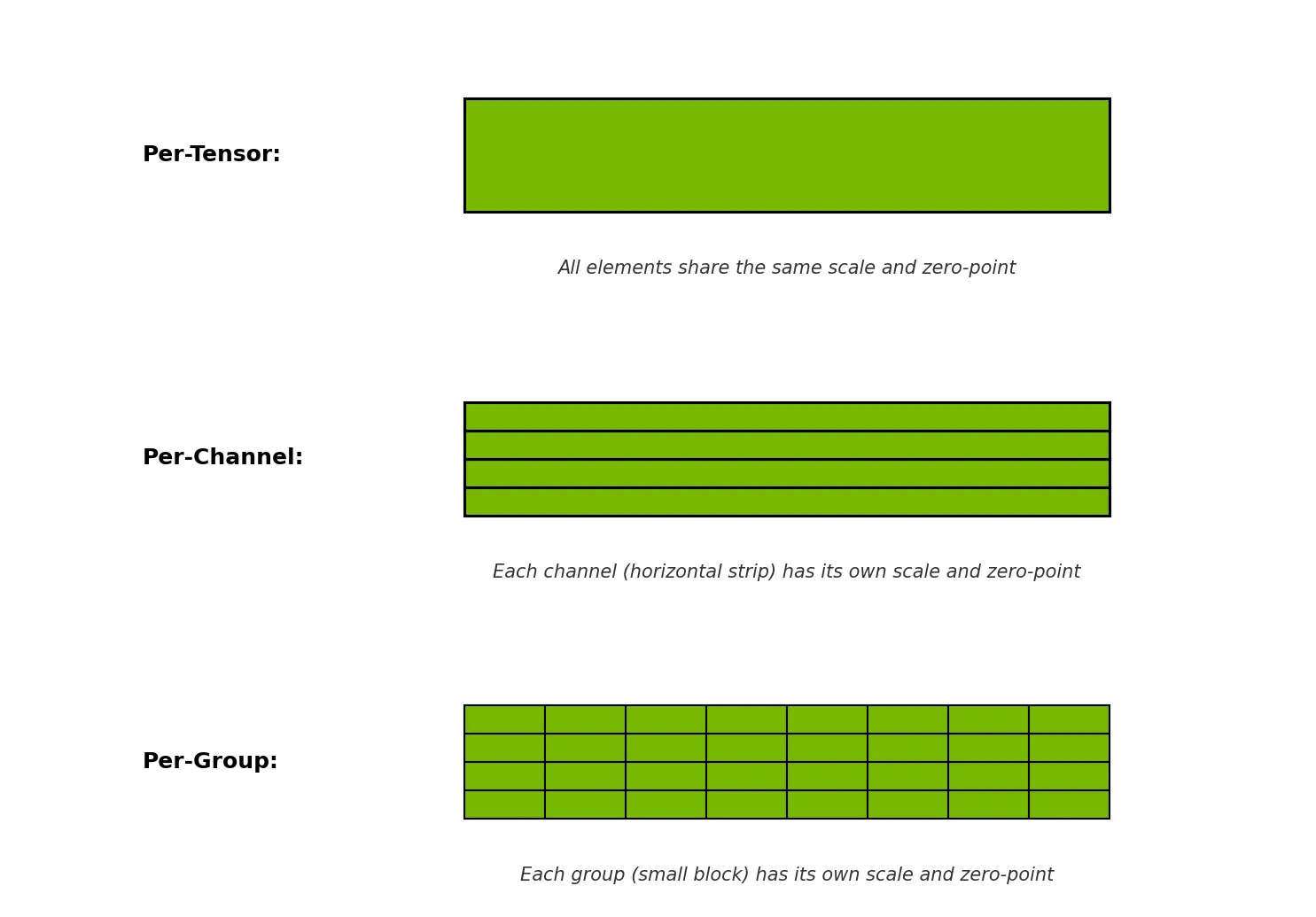
Per-tensor quantization
One scale factor for the entire tensor. Simplest approach, minimal memory overhead for storing quantization parameters. But if different parts of the tensor have wildly different value distributions, you're forcing a single compromise that hurts everywhere.
Per-channel quantization
Separate scale factors for each channel (typically along the output dimension of a weight matrix). This isolates outlier channels: one channel with extreme values no longer drags down the precision of all other channels. The overhead is small (one extra float per channel) and the accuracy improvement is usually significant.
Per-block (per-group) quantization
Divide the tensor into fixed-size blocks (e.g., groups of 128 values) and compute separate quantization parameters for each block. This is the finest granularity in common use and gives the best accuracy, at the cost of storing more scale factors and slightly more complex kernel implementations.
I learned this the hard way. My first attempt at quantizing a model used per-tensor quantization because it was the default in the framework I was using. Accuracy dropped by 3 percentage points. Switching to per-channel quantization recovered almost all of it. The lesson: before tweaking algorithms, check your granularity setting.
Advanced quantization algorithms
AbsMax gets you 80% of the way there. The remaining 20%, the difference between "works fine" and "production-ready", comes from algorithms that are more careful about which values matter most.
AWQ: activation-aware weight quantization
AWQ observes that not all weight channels contribute equally to model output. A small fraction, typically 1% or less, are disproportionately important, and these tend to correspond to large activation magnitudes.
The idea: instead of treating all weights equally, AWQ identifies "salient" channels by examining activation statistics from a calibration dataset. It then applies per-channel scaling to protect these important weights before quantization. Multiply important weight channels by a scaling factor greater than 1 before quantization, then divide the corresponding activation channels by the same factor to maintain mathematical equivalence:
This is a weight-only method, and it's become one of the most popular approaches for deploying large language models at INT4 precision.
GPTQ: generative pre-trained transformer quantization
GPTQ takes a different approach. It quantizes each row of a weight matrix independently, using approximate second-order information (the Hessian matrix) to decide how to round each weight. The core idea: when you quantize one weight, the rounding error propagates to the output, so you should adjust the remaining unquantized weights to compensate.
This "optimal brain quantization" approach was originally proposed for network pruning and later adapted for quantization. GPTQ can quantize a 175B parameter model in roughly 4 hours on a single GPU. Fast enough to be practical, and the accuracy loss is minimal compared to the uncompressed model.
SmoothQuant
SmoothQuant targets a different problem entirely. Weight distributions are usually well-behaved, roughly Gaussian, centred around zero. But activation distributions often have severe outliers in specific channels. These outliers make activation quantization difficult because the scale factor gets inflated by extreme values.
SmoothQuant's solution: mathematically shift the quantization difficulty from activations to weights by applying a per-channel scaling transformation before quantization:
The scaling factor is chosen to smooth out activation outliers (hence the name). After smoothing, both weights and activations can be quantized to INT8 without significant accuracy loss, enabling W8A8 quantization (8-bit weights and 8-bit activations).
Post-training quantization vs. quantization-aware training
There are two approaches to when you apply quantization: after training is complete (PTQ), or during training itself (QAT).
Post-training quantization (PTQ)
PTQ is the pragmatic choice. You take a pre-trained model and quantize it without any additional training. For weight-only quantization, you don't even need data: the weights are static and can be mapped directly. For activations, you need a small calibration dataset to observe the activation distributions and compute appropriate scale factors.
PTQ comes in two flavours:
Static quantization: run the calibration dataset through the model once, compute scale factors for all activations, and fix them permanently. Every future inference uses the same quantization parameters.
Dynamic quantization: compute activation quantization parameters on the fly during each inference pass. No calibration dataset needed, and the parameters adapt to each input. The cost is extra computation at inference time to calculate the scales.
For most deployment scenarios, static PTQ with a representative calibration dataset of a few hundred samples is the right starting point. It's fast, it's simple, and the accuracy loss is typically small.
Quantization-aware training (QAT)
QAT is the expensive insurance policy you reach for when PTQ isn't good enough. Instead of quantizing after training, QAT simulates quantization effects during training by inserting "fake quantization" modules that quantize and immediately dequantize values in the forward pass:
The model trains with these simulated quantization effects, so its parameters learn to tolerate the rounding and clipping errors that quantization introduces. The actual computation during training still happens in full precision. The fake quantization modules just add noise that mimics what real quantization would do.
There's a technical wrinkle: the function has zero gradient almost everywhere, which breaks backpropagation. QAT works around this using the Straight-Through Estimator (STE), which approximates the gradient of the rounding function as 1, pretending the rounding didn't happen during the backward pass:
Mathematically dubious. Empirically effective. QAT consistently outperforms PTQ on accuracy, especially for aggressive quantization (INT4, INT2). The cost is that you need the training infrastructure, the training data, and the compute budget to fine-tune the model, which is why PTQ remains the default for most of us.
What I actually use
After working through all of this and breaking enough models in practice, here's where I've landed:
Start with per-channel symmetric PTQ at INT8. It covers 90% of use cases with minimal accuracy loss. TensorRT defaults to this, and there's a reason for that.
If memory is the bottleneck, try INT4 with AWQ or GPTQ. Weight-only INT4 halves your memory again with surprisingly little accuracy degradation for LLMs. AWQ is simpler. GPTQ gives slightly better results on some models.
If you need both fast and accurate, look at SmoothQuant for W8A8. Quantizing both weights and activations gives you the full speedup from tensor core acceleration, and SmoothQuant handles the activation outlier problem well enough for production.
Reserve QAT for when PTQ measurably fails. If your accuracy metrics drop below acceptable thresholds with PTQ, and you have the compute budget, QAT will usually recover 50-80% of the lost accuracy. But it's expensive. Budget the same resources as a full fine-tuning run.
And always measure what actually matters. Perplexity and accuracy benchmarks are necessary but not sufficient. Measure latency (both cold and warm start), peak memory usage, and end-to-end throughput on your actual deployment hardware. A model that's 0.5% more accurate but 2× slower isn't a better model. It's a worse system.
References
Lin, J., Tang, J., Tang, H., Yang, S., Chen, W.-M., Wang, W.-C., Xiao, G., Dang, X., Gan, C., & Han, S. (2024). AWQ: Activation-aware weight quantization for LLM compression and acceleration. Proceedings of Machine Learning and Systems, 6, 87–100. https://arxiv.org/abs/2306.00978
Frantar, E., Ashkboos, S., Hoefler, T., & Alistarh, D. (2023). GPTQ: Accurate post-training quantization for generative pre-trained transformers. International Conference on Learning Representations. https://arxiv.org/abs/2210.17323
Xiao, G., Lin, J., Seznec, M., Wu, H., Demouth, J., & Han, S. (2023). SmoothQuant: Accurate and efficient post-training quantization for large language models. Proceedings of the 40th International Conference on Machine Learning. https://arxiv.org/abs/2211.10438
Bengio, Y., Léonard, N., & Courville, A. (2013). Estimating or propagating gradients through stochastic neurons for conditional computation. arXiv preprint arXiv:1308.3432. https://arxiv.org/abs/1308.3432
Wang, R. (2025). Model quantization: Concepts, methods, and why it matters. NVIDIA Developer Blog. https://developer.nvidia.com/blog/model-quantization-concepts-methods-and-why-it-matters/

Discussion (0)
Sign in to join the discussion.